Policy adaptation after an environment change

This case shows how an agent uses DEVS-Gen to build a supply-chain simulator, choose a replenishment policy, and adapt that policy after operating conditions change. The task is to decide how much stock stores and warehouses should order to minimize inventory holding and backlog costs over 100 days.

The starting input is a written description of the supply network, initial inventories, delivery lead times, demand and costs. DEVS-Gen turns this description into an executable simulator; the agent uses its feedback to compare candidate policies. The materials below show the specifications, simulator code, policy choices, operating records and final cost evaluation.

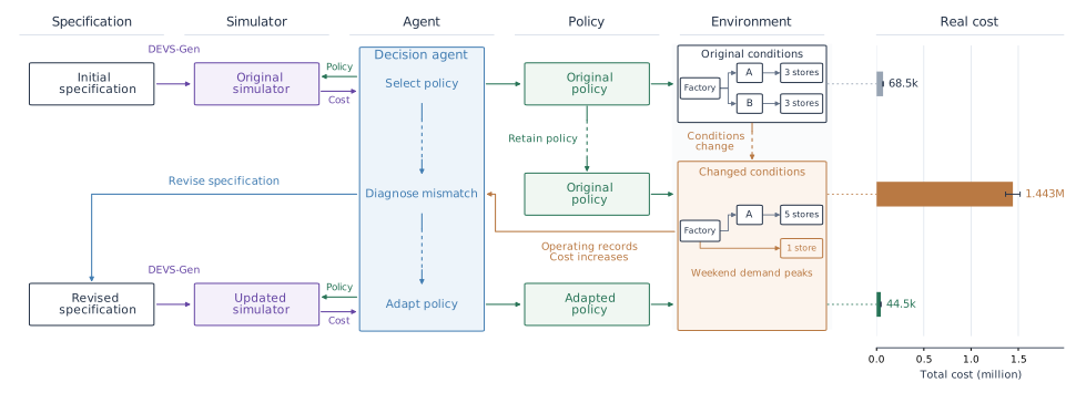
Five columns trace specifications, simulators, one decision agent, policies and the changing supply environment. Three horizontal Real cost bars align with the policy/environment combinations.

The figure follows specifications, simulators, the decision agent, policies and the operating environment from left to right. Its three rows show the initial decision, the effect of changed conditions, and the adapted decision.

  1. Build the first policy. A factory initially serves six stores through two warehouses. DEVS-Gen constructs the initial simulator from the description, and the agent tests candidate replenishment rules to select the first policy.
  2. Use operating feedback to update the model. One warehouse closes, its stores are reassigned, and one store switches to direct factory supply with weekday/weekend demand. The original policy becomes costly under these conditions. Operating records and the confirmed changes inform a revised specification, which DEVS-Gen uses to construct the updated simulator.
  3. Select and evaluate an adapted policy. The agent compares candidates using the updated simulator and selects a new policy. The bars compare real costs for the original policy in the original environment, the original policy in the changed environment, and the adapted policy in the changed environment.

Final evaluation uses the same 20 environment seeds and 100 days per episode. In the changed environment, mean real cost falls from 1,442,662.51 with the original policy to 44,491.23 with the adapted policy, a 96.92% reduction. Error bars show sample standard deviations across seeds.

Case timeline and materials

Follow the case from the initial environment description to the first policy, then through operating feedback, simulator updates and policy adaptation. Each step identifies its inputs and outputs.

  1. Begin with the environment description

    The case starts with a description of the supply network and a replenishment objective. The first simulator and policy are developed from this starting point.

    Provided input

    Initial environment description

    A factory supplies six stores through two warehouses. The description specifies initial stock, lead times, demand variability and holding/backlog costs.

    Provided task

    Choose a replenishment policy

    Design retailer and warehouse order rules to minimize total holding and backlog cost over a 100-day episode.

    Read the initial environment specification
    NETWORK AND INITIAL STATE
    Factory → warehouse A → stores 0–2; Factory → warehouse B → stores 3–5.
    Each warehouse starts with 800 units; each store starts with 100. Factory supply is unlimited.
    Factory-to-warehouse lead time: 4 days. Warehouse-to-store lead time: 2 days.
    
    DEMAND AND COST
    Every store: max(0, 25 + Uniform(−8, 8) + 5 sin(2π day / 14)).
    Store holding/backlog costs: 3 / 120 per unit per day.
    Warehouse holding/backlog costs: 0.8 / 40. Unsatisfied demand is backlogged.
    Costs accrue at day end; no terminal salvage value.
    
    POLICY INTERFACE
    period is 1-based; inventory_dict = {1: inventory_position}.
    Inventory position = on-hand + all outstanding replenishment orders − backlog.
    Policies return a nonnegative quantity through POLICY_MOUNTS.
    Evaluation episodes start from the stated initial stock, with zero backlog/pipeline.
  2. Build the initial simulator

    DEVS-Gen turns the environment description into a component model that can execute candidate replenishment policies and return costs.

    Construction input

    Network, demand and cost rules

    The initial specification defines how inventory, outstanding orders, deliveries and unmet demand evolve over time.

    Construction output

    Initial DEVS simulator

    The model implements the original two-warehouse environment and exposes the policy interface used for decision-making.

    Inspect the initial component hierarchy
    FixedSupply02
      SimulationRuntime
      SupplyChainNetwork
        DemandSequencer
        RetailLayer
          RetailerNode
        FactoryNode
        TemporalEventJoiner
        DistributionLayer
          RegionalDcNode
  3. Test candidates and output the first policy

    The agent uses simulator feedback to compare replenishment rules in the initial environment, then selects the first policy before it is deployed.

    Simulator feedback

    Initial candidate comparison

    The archived setup search tested two candidates over 100 days with development seed 42. Candidate A cost 71,307.76, compared with 173,596.53 for B.

    Agent output

    First policy · candidate A

    Candidate A is the selected replenishment policy. This exact policy becomes the original policy used in the operating records and subsequent comparisons.

    Read the first policy and inventory targets
    import math
    
    def retailer_policy_func(period: int, inventory_dict: dict) -> dict:
        ip = float(inventory_dict.get(1, 0.0))
        seasonal = 5.0 * math.sin(2.0 * math.pi * period / 14.0)
        # Two-day lead time plus one review day and a moderate uncertainty buffer.
        target = 25.0 * 3.0 + seasonal * 2.0 + 22.0
        qty = max(0.0, target - ip)
        order = {1: qty}
        return {"Regional_DC_0": order, "Regional_DC_1": {1: qty}}
    
    def dc_policy_func(period: int, inventory_dict: dict) -> dict:
        ip = float(inventory_dict.get(1, 0.0))
        seasonal = 5.0 * math.sin(2.0 * math.pi * period / 14.0)
        # Four-day factory lead time, covering the three downstream retailers.
        target = 25.0 * 3.0 * 5.0 + seasonal * 3.0 + 140.0
        qty = max(0.0, target - ip)
        return {"Factory_0": {1: qty}}
    
    POLICY_MOUNTS = {
        "Retailer": retailer_policy_func,
        "Regional_DC": dc_policy_func,
    }
    

    The retailer target covers three days of mean demand plus a seasonal allowance and 22 units of safety stock. Each warehouse covers five days of demand for its three stores, plus a seasonal allowance and 140 units.

    Inspect the archived initial policy search

    The first policy was selected in the earlier setup run and is reused unchanged in the later adaptation recording.

    Initial candidateSimulator cost · seed 42Decision
    Candidate A71,307.76Selected as the first policy
    Candidate B173,596.53
  4. Inspect operating records and diagnose the mismatch

    The same policy is observed under the original and changed conditions. The agent uses these records to identify what needs checking.

    Input to agent · observe_operation

    28-day operating records

    Total cost rises from 24,129.11 to 232,398.95. The records include store demand, inventory and backlog costs.

    Agent output

    Diagnosis and request for confirmation

    The new deployment has one warehouse, widespread warehouse-driven shortages, and a changed demand pattern at Retailer_5. Confirm topology, lead times, calendars, demand laws, and initial stocks before rebuilding the simulator or testing policies.
    Inspect the operating costs and daily records
    28-day operationHolding costBacklog costTotal cost
    Original environment24,129.110.0024,129.11
    Changed environment18,725.91213,673.05232,398.95
    DayDemand: originalDemand: changedStock: originalStock: changedBacklog cost: changed
  5. Confirm the changes and specify the new model

    The agent requests the operational change bulletin, then turns the confirmed rules into a DEVS-Gen construction request.

    Tool response · inspect_change_report

    Confirmed operating rules

    • Warehouse B closes; A supplies five stores and receives B’s initial stock.
    • The sixth store becomes factory-direct, with a 3-day lead time.
    • That store’s demand changes to a weekday/weekend pattern.

    Agent output · devs_gen request

    Revised simulator requirements

    The request specifies the new topology, lead times, demand rules and initial state, together with event ordering and cost accounting.

    Read the agent-written business requirements (excerpt)
    Revised topology: unlimited Factory_0 supplies only Regional_DC_0 and direct Retailer_5; Regional_DC_1 is closed and absent. Regional_DC_0 supplies Retailer_0 through Retailer_4. Factory_0 to Regional_DC_0 lead time 4 days; Regional_DC_0 to Retailer_0..4 lead time 2 days; Factory_0 to Retailer_5 lead time 3 days. Each episode begins independently on day 1 Monday, Regional_DC_0 on-hand 1600, all six retailers on-hand 100, all backlogs and outstanding orders/pipelines zero. This is not migration of a running snapshot. For each day, generate exactly one demand draw per retailer in index order 0..5 using a single random.Random(seed). Retailer_0..4 demand=max(0,25+Uniform(-8,8)+5*sin(2*pi*day/14)); independent draws. Retailer_5 demand=max(0,20+Uniform(-4,4)) Monday-Friday, max(0,40+Uniform(-4,4)) Saturday-Sunday; day 1 Monday. All unmet demand/orders are backlogged, not lost; enforce conservation and retain unfilled replenishment orders in inventory position until fulfilled. Charge day-end retailer on-hand holding 3/unit/day and backlog 120/unit/day; warehouse on-hand holding 0.8/unit/day and backlog 40/unit/day. No salvage, transport, ordering costs or supply limits at factory.
    Read the revised environment summary
    SUPPLY NETWORK
    Warehouse B closes; its initial 800 units transfer to A, which starts with 1,600.
    A serves stores 0–4. Store 5 receives directly from the factory with a 3-day lead time.
    Other lead times and each store’s initial stock remain unchanged.
    
    DEMAND
    Stores 0–4 retain the original random seasonal demand.
    Store 5: max(0, 20 + Uniform(−4, 4)) on weekdays;
             max(0, 40 + Uniform(−4, 4)) on weekends. Day 1 is Monday.
    Each day, one RNG draws demands for stores 0–5 in that order.
    
    DECISION TASK
    Adapt replenishment to the shared warehouse load and direct-store demand.
    The original quantity rule is retained for comparison; a common adapter maps it to the current suppliers.
    Cost rules and policy inputs retain their original definitions.
  6. Return an updated executable simulator

    DEVS-Gen constructs a model for the revised specification. This model is then reused to test candidate policies.

    Input to DEVS-Gen

    Revised specification

    The construction request from step 5 describes a complete 100-day episode with the changed network and demand mechanism.

    Tool output

    Updated simulator and PlanTree

    The simulator exposes the policy interface used in the next step.

    Browse the simulator source and construction files

  7. Test candidate policies and select one

    The agent submits five policies to the updated simulator, reads the cost feedback and selects candidate c1.

    Simulator output · run_simulator

    Candidate cost feedback

    Each candidate runs on development seeds 42 and 7. Candidate c1 has the lowest mean simulator cost: 46,128.65.

    Agent output · save_policy

    Selected policy c1

    The policy adjusts warehouse coverage and gives the direct store a separate weekday/weekend demand forecast.

    Compare all five candidates
    CandidateSeed 42Seed 7Mean simulator costSelection
    c147,381.7144,875.5946,128.65Selected
    c248,497.9549,181.3948,839.67
    c349,239.1645,964.9847,602.07
    c453,166.4048,908.1051,037.25
    c546,858.8946,266.7046,562.79
    Read the selected policy and replenishment targets
    import math
    
    def mean_demand(day):
        return 25.0 + 5.0 * math.sin(2.0 * math.pi * day / 14.0)
    
    def retailer_policy_func(period, inventory_dict):
        if period > 98:
            return {1: 0.0}
        target = sum(mean_demand(d) for d in range(period, min(100, period + 2) + 1)) + 16.0
        return {1: max(0.0, target - float(inventory_dict.get(1, 0.0)))}
    
    def dc_policy_func(period, inventory_dict):
        if period > 94:
            return {1: 0.0}
        target = 5.0 * sum(mean_demand(d + 2) for d in range(period, min(98, period + 4) + 1)) + 45.0
        return {1: max(0.0, target - float(inventory_dict.get(1, 0.0)))}
    
    def direct_retailer_policy_func(period, inventory_dict):
        if period > 97:
            return {1: 0.0}
        target = sum(40.0 if (d - 1) % 7 >= 5 else 20.0 for d in range(period, min(100, period + 3) + 1)) + 9.0
        return {1: max(0.0, target - float(inventory_dict.get(1, 0.0)))}
    
    POLICY_MOUNTS = {'Retailer': retailer_policy_func, 'Regional_DC': dc_policy_func, 'Direct_Retailer': direct_retailer_policy_func}
    
    RoleDemand coverageSafety allowance
    Ordinary store3 days of seasonal demand16 units
    Direct store4 days using weekday/weekend demand9 units
    Warehouse A5 days across five stores, shifted by the store lead time45 units

    The policy also stops orders that cannot arrive before the 100-day horizon.

  8. Evaluate the selected policy in the changed environment

    After selection, Stockpyl measures real cost on 20 common environment seeds (1000–1019), with 100 days per episode from the specified initial state.

    Evaluation inputs: frozen original and selected policiesMeasured output: real cost, mean ± sample SD
    Policy / environmentReal cost (mean ± SD)
    Original policy / original environment68,540.25 ± 1,410.42
    Original policy / changed environment1,442,662.51 ± 76,818.26
    Adapted policy / changed environment44,491.23 ± 1,920.36

    In the changed environment, the selected policy reduces mean real cost by 96.92% relative to the original policy.

    All 20 environment seeds
    SeedOriginal / originalOriginal / changedAdapted / changed
    100067,411.991,464,903.0744,771.31
    100167,340.431,427,520.3241,638.08
    100269,217.231,501,873.6644,058.30
    100368,026.841,458,577.8244,481.01
    100467,461.031,587,425.5443,514.15
    100566,983.531,523,776.9044,386.37
    100668,395.811,431,106.3542,761.09
    100768,403.761,447,877.2547,804.62
    100869,341.571,413,988.2245,086.32
    100970,200.191,348,863.9546,098.21
    101068,626.161,388,926.8249,085.68
    101171,700.071,334,978.4344,210.22
    101268,584.741,417,317.7243,735.75
    101368,017.871,429,586.4141,810.30
    101470,301.911,317,428.6644,628.33
    101567,125.101,483,886.6744,586.19
    101670,782.101,324,496.8243,578.56
    101765,963.221,583,690.2443,460.93
    101868,837.951,468,503.0647,540.57
    101968,083.491,498,522.3042,588.55
Adaptation walkthrough · 9 tool calls

This recording covers the adaptation phase, from operating feedback to updated simulator construction and policy selection. The decision agent is gpt-6.1-sol.

  1. observe_operation

    Inspect the deployed policy’s forecasts, actual operating records, demands, and initial conditions before identifying policy or model changes.

    28-day forecasts and operating records returned.

    Tool input (excerpt)
    {}
  2. inspect_change_report

    The new deployment has one warehouse, widespread warehouse-driven shortages, and a changed demand pattern at Retailer_5. Confirm topology, lead times, calendars, demand laws, and initial stocks before rebuilding the simulator or testing policies.

    Supply routes, replenishment lead times and demand rules confirmed.

    Tool input (excerpt)
    {}
  3. devs_gen

    Confirmed changes alter warehouse coverage, direct-store lead time, and weekend demand. Rebuild the environment to evaluate revised policies.

    Updated simulator returned.

    Tool input (excerpt)
    {
      "requirements": "Construct a complete revised supply-network DEVS simulator for 100-day independent episodes, seeds 42 and 7, preserving the existing validated simulator's within-day event ordering, lead-time interpretation, shipment allocation/backlog fulfillment conventions, and policy invocation semantics. Revised topology: unlimited Factory_0 supplies only Regional_DC_0 and direct Retailer_5; Regional_DC_1 is closed and absent. Regional_DC_0 supplies Retailer_0 through Retailer_4. Factory_0 to Regional_DC_0 lead time 4 days; Regional_DC_0 to Retailer_0..4 lead time 2 days; Factory_0 to Retailer_5 lead time 3 days. Each episode begins independently on day 1 Monday, Regional_DC_0 on-hand 1600, all six retailers on-hand 100, all backlogs and outstanding orders/pipelines zero. This is not migration of a running snapshot. For each day, generate exactly one demand draw per retailer in index order 0..5 using a single random.Random(seed). Retailer_0..4 demand=max(0,25+Uniform(-8,8)+5*sin(2*pi*day/14)); independent draws. Retailer_5 demand=max(0,20+Uniform(-4,4)) Monday-Friday, max(0,40+Uniform(-4,4)) Saturday-Sunday; day 1 Monday. All unmet demand/orders are backlogged, not lost; enforce conservation and retain unfilled replenishment orders in inventory position until fulfilled. Charge day-end retailer on-hand holding 3/unit/day and backlog 120/unit/day; warehouse on-hand holding 0.8/unit/day and backlog 40/unit/day. No salvage, transport, ordering costs or supply limits at factory. Objective total holding plus backlog costs over days 1..100; report each seed and aggregate, preferably retailer/warehouse breakdown. Policy receives period integer 1..100 and plain inventory_dict={1:inventory_position}, where inventory_position=on-hand+all outstanding replenishment orders-backlog, after incoming receipts but before new downstream orders/demand. Policies return {1:quantity} or {'UPSTREAM':{1:quantity}}; common adapter routes to actual supplier and mechanically reroutes legacy supplier keys without optimizing quantities. POLICY_MOUNTS must support Retailer and Regional_DC and optionally Direct_Retailer, defaulting Direct_Retailer to Retailer if absent. Expose accepted revised model to run_simulator. Verify topology, calendars, initial stocks, exact RNG draw ordering, lead-time/event semantics, conservation/backlogs and day-end accounting. Existing operating evidence is diagnostic, not a replacement for these confirmed business rules."
    }
  4. run_simulator · c1

    Test a policy covering all five warehouse-served stores, forecasting ordinary seasonal demand across lead time plus review, and giving the direct store its own four-day weekday/weekend forecast. Stop orders that cannot arrive within the horizon.

    c1: mean simulator cost 46,128.65 over seeds 42 and 7.

    Tool input (excerpt)
    {
      "candidate_id": "c1",
      "code": "import math\n\ndef mean_demand(day):\n    return 25.0 + 5.0 * math.sin(2.0 * math.pi * day / 14.0)\n\ndef retailer_policy_func(period, inventory_dict):\n    if period > 98:\n        return {1: 0.0}\n    target = sum(mean_demand(d) for d in range(period, min(100, period + 2) + 1)) + 16.0\n    return {1: max(0.0, target - float(inventory_dict.get(1, 0.0)))}\n\ndef dc_policy_func(period, inventory_dict):\n    if period > 94:\n        return {1: 0.0}\n    target = 5.0 * sum(mean_demand(d + 2) for d in range(period, min(98, period + 4) + 1)) + 45.0\n    return {1: max(0.0, target - float(inventory_dict.get(1, 0.0)))}\n\ndef direct_retailer_policy_func(period, inventory_dict):\n    if period > 97:\n        return {1: 0.0}\n    target = sum(40.0 if (d - 1) % 7 >= 5 else 20.0 for d in range(period, min(100, period + 3) + 1)) + 9.0\n    return {1: max(0.0, target - float(inventory_dict.get(1, 0.0)))}\n\nPOLICY_MOUNTS = {'Retailer': retailer_policy_func, 'Regional_DC': dc_policy_func, 'Direct_Retailer': direct_retailer_policy_func}\n"
    }
  5. run_simulator · c2

    Candidate c1 averaged 46,128.65 over the two 100-day seeds, with substantial remaining backlog cost. Test larger warehouse and ordinary-store buffers to determine whether better service offsets extra holding cost.

    c2: mean simulator cost 48,839.67 over seeds 42 and 7.

    Tool input (excerpt)
    {
      "candidate_id": "c2",
      "code": "import math\n\ndef mean_demand(day):\n    return 25.0 + 5.0 * math.sin(2.0 * math.pi * day / 14.0)\n\ndef retailer_policy_func(period, inventory_dict):\n    if period > 98:\n        return {1: 0.0}\n    target = sum(mean_demand(d) for d in range(period, min(100, period + 2) + 1)) + 18.0\n    return {1: max(0.0, target - float(inventory_dict.get(1, 0.0)))}\n\ndef dc_policy_func(period, inventory_dict):\n    if period > 94:\n        return {1: 0.0}\n    target = 5.0 * sum(mean_demand(d + 2) for d in range(period, min(98, period + 4) + 1)) + 90.0\n    return {1: max(0.0, target - float(inventory_dict.get(1, 0.0)))}\n\ndef direct_retailer_policy_func(period, inventory_dict):\n    if period > 97:\n        return {1: 0.0}\n    target = sum(40.0 if (d - 1) % 7 >= 5 else 20.0 for d in range(period, min(100, period + 3) + 1)) + 9.0\n    return {1: max(0.0, target - float(inventory_dict.get(1, 0.0)))}\n\nPOLICY_MOUNTS = {'Retailer': retailer_policy_func, 'Regional_DC': dc_policy_func, 'Direct_Retailer': direct_retailer_policy_func}\n"
    }
  6. run_simulator · c3

    Candidate c2 reduced backlog penalties but raised mean total cost to 48,839.67. Test a smaller ordinary-store buffer and intermediate warehouse buffer to balance expensive store stock against pooled upstream protection.

    c3: mean simulator cost 47,602.07 over seeds 42 and 7.

    Tool input (excerpt)
    {
      "candidate_id": "c3",
      "code": "import math\n\ndef mean_demand(day):\n    return 25.0 + 5.0 * math.sin(2.0 * math.pi * day / 14.0)\n\ndef retailer_policy_func(period, inventory_dict):\n    if period > 98:\n        return {1: 0.0}\n    target = sum(mean_demand(d) for d in range(period, min(100, period + 2) + 1)) + 14.0\n    return {1: max(0.0, target - float(inventory_dict.get(1, 0.0)))}\n\ndef dc_policy_func(period, inventory_dict):\n    if period > 94:\n        return {1: 0.0}\n    target = 5.0 * sum(mean_demand(d + 2) for d in range(period, min(98, period + 4) + 1)) + 60.0\n    return {1: max(0.0, target - float(inventory_dict.get(1, 0.0)))}\n\ndef direct_retailer_policy_func(period, inventory_dict):\n    if period > 97:\n        return {1: 0.0}\n    target = sum(40.0 if (d - 1) % 7 >= 5 else 20.0 for d in range(period, min(100, period + 3) + 1)) + 9.0\n    return {1: max(0.0, target - float(inventory_dict.get(1, 0.0)))}\n\nPOLICY_MOUNTS = {'Retailer': retailer_policy_func, 'Regional_DC': dc_policy_func, 'Direct_Retailer': direct_retailer_policy_func}\n"
    }
  7. run_simulator · c4

    Candidate c3 increased backlog costs and averaged 47,602.07. Test 18 units of ordinary-store safety stock with a leaner 30-unit warehouse buffer; c1 remains the best tested candidate at 46,128.65.

    c4: mean simulator cost 51,037.25 over seeds 42 and 7.

    Tool input (excerpt)
    {
      "candidate_id": "c4",
      "code": "import math\n\ndef mean_demand(day):\n    return 25.0 + 5.0 * math.sin(2.0 * math.pi * day / 14.0)\n\ndef retailer_policy_func(period, inventory_dict):\n    if period > 98:\n        return {1: 0.0}\n    target = sum(mean_demand(d) for d in range(period, min(100, period + 2) + 1)) + 18.0\n    return {1: max(0.0, target - float(inventory_dict.get(1, 0.0)))}\n\ndef dc_policy_func(period, inventory_dict):\n    if period > 94:\n        return {1: 0.0}\n    target = 5.0 * sum(mean_demand(d + 2) for d in range(period, min(98, period + 4) + 1)) + 30.0\n    return {1: max(0.0, target - float(inventory_dict.get(1, 0.0)))}\n\ndef direct_retailer_policy_func(period, inventory_dict):\n    if period > 97:\n        return {1: 0.0}\n    target = sum(40.0 if (d - 1) % 7 >= 5 else 20.0 for d in range(period, min(100, period + 3) + 1)) + 9.0\n    return {1: max(0.0, target - float(inventory_dict.get(1, 0.0)))}\n\nPOLICY_MOUNTS = {'Retailer': retailer_policy_func, 'Regional_DC': dc_policy_func, 'Direct_Retailer': direct_retailer_policy_func}\n"
    }
  8. run_simulator · c5

    Use the fifth and final candidate to retain c1's ordinary-store and direct-store settings while increasing its warehouse buffer from 45 to 65. This isolates whether moderate additional warehouse protection reduces total cost; select the lowest measured mean afterward.

    c5: mean simulator cost 46,562.79 over seeds 42 and 7.

    Tool input (excerpt)
    {
      "candidate_id": "c5",
      "code": "import math\n\ndef mean_demand(day):\n    return 25.0 + 5.0 * math.sin(2.0 * math.pi * day / 14.0)\n\ndef retailer_policy_func(period, inventory_dict):\n    if period > 98:\n        return {1: 0.0}\n    target = sum(mean_demand(d) for d in range(period, min(100, period + 2) + 1)) + 16.0\n    return {1: max(0.0, target - float(inventory_dict.get(1, 0.0)))}\n\ndef dc_policy_func(period, inventory_dict):\n    if period > 94:\n        return {1: 0.0}\n    target = 5.0 * sum(mean_demand(d + 2) for d in range(period, min(98, period + 4) + 1)) + 65.0\n    return {1: max(0.0, target - float(inventory_dict.get(1, 0.0)))}\n\ndef direct_retailer_policy_func(period, inventory_dict):\n    if period > 97:\n        return {1: 0.0}\n    target = sum(40.0 if (d - 1) % 7 >= 5 else 20.0 for d in range(period, min(100, period + 3) + 1)) + 9.0\n    return {1: max(0.0, target - float(inventory_dict.get(1, 0.0)))}\n\nPOLICY_MOUNTS = {'Retailer': retailer_policy_func, 'Regional_DC': dc_policy_func, 'Direct_Retailer': direct_retailer_policy_func}\n"
    }
  9. save_policy

    All five permitted candidates have been tested. Save c1 because it achieved the lowest observed mean total cost under the accepted revised environment.

    Selected policy c1.

    Tool input (excerpt)
    {
      "candidate_id": "c1",
      "explanation": "Select c1, the lowest-cost of all five tested candidates over 100-day independent episodes with seeds 42 and 7. Mean holding-plus-backlog costs: c1 46128.65, c2 48839.67, c3 47602.07, c4 51037.25, c5 46562.79. The selected policy accounts for five ordinary stores supplied by the consolidated warehouse, uses seasonal demand forecasts with 16-unit store and 45-unit warehouse buffers, and mounts a separate direct-store policy covering the three-day lead time plus review with weekday/weekend demand and a 9-unit buffer. It stops replenishment orders that cannot arrive within the horizon. These results support selection among the tested candidates; no independent final evaluation or same-environment test of the original policy was available, so no global optimality or quantified improvement over the original policy is claimed."
    }